Case Studies

A step by step guide to the code for the three case studies presented in our paper (to come).

Contents

Bottle Experiment
Global Steady state
Nitrogen Fixers Niche

Before you begin

If you haven't already, follow the getting started instructions, which will guide you through installation, general program structure, and workflow.

This guide to the case studies assumes you are using docker or otherwise working from a command line. If you would rather have a graphical interface, you can use the Docker extension in VS Code.

For each case study, there is a build file and a run file. These instructions will have you open each file, explain the contents, then close it and execute it with the julia command from the command line.

If you are using the docker, you can find the code for the case students in the /dar_one_docker/Dar_One/case_studies directory.

cd /dar_one_docker/Dar_One/case_studies
ls

You should see the following six files listed.

bottle_experiment_build.jl
bottle_experiment_run.jl
global_steadystate_build.jl
global_steadystate_run.jl
nitrogen_fixers_run.jl
nitrogen_fixers_build.jl

You can also find the code on github here.

Each case study has a file to build the Darwin model and a file to run it. As explained in the getting started document, you only need to run the build step when making structural changes to your experiments - such as a new grid size, setting ambient nutrients to be constant or cycling, or a new number of plankton tracers. After building once, you can change other parameters from run to run without building again - such as nutrient levels, plankton abundances, temperature, and light.

Case Study A - Bottle Experiment

A simple nutrient amendment experiment. What happens if we take a plankton community that is nitrogen limited and add nitrogen?

Overview

In this experiment, DAR1 is initialized with values from a global DARWIN run. Initial parameter values were taken from location X=203 and Y=108 (lon = 203.5, lat = 28.5). In the control run, nothing was modified. For the bottle experiment run, nitrate values were increased 10x.

bottle experiment

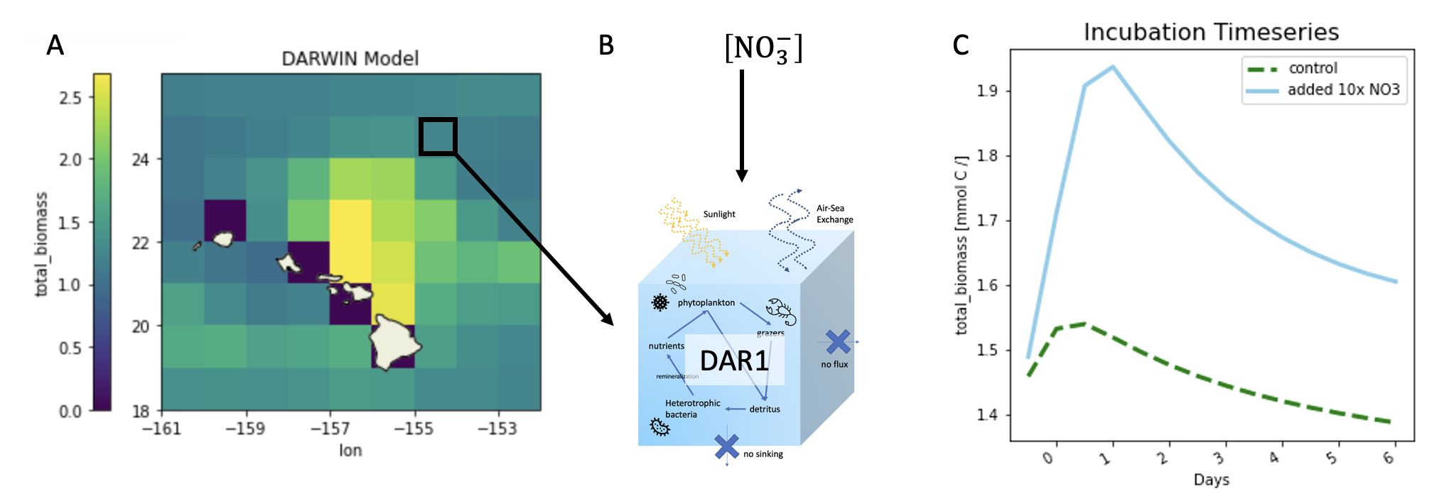
The initial parameters that were set include all nutrient tracers (TRAC01-TRAC20), all biomass tracers excluding diazotrophs (TRAC21-TRAC29, TRAC35-TRAC70), PAR at a depth of 45m, and temperature. It was set to run for 7 days (56 iterations), writing to diagnostic files every 4 hours (14400 seconds). Reminder that you can find a list of all nutrient and plankton tracers in Darwin background

Code Walkthrough

From the Docker command line, we can open up the bottleexperimentbuild.jl file using the following command

vim bottle_experiment_build.jl

Reminder that we are in the /dar_one_docker/Dar_One/case_studies directory. Use the arrow keys to navigate the cursor around with vim, i to enter insert mode, esc to exit the mode, and :q to close the file. We will walk through all the code in this file before running it.

You will see these lines of code at the top of the file.

include("../src/DarOneTools.jl")
using .DarOneTools
# other packages 
using ClimateModels
using NCDatasets

This loads up DarOneTools, then imports it along with the ClimateModels and NCDatasets packages. You will see these lines of code repeated at the top of every file we work with from here on out!

Next we have to let MITgcm_path[1] point to the directory where the Darwin Fortran code lives, establish that we are working with a 1x1 parcel of water (instead of running multiple grid cells at once), and we want to allow all nutrients to freely cycle (intead of holding the concentrations in the water constant).

Note that if you are not using Docker, you will have to change the MITgcm_path[1] = "directory/to/darwin" line of code to contain the directory in which the Darwin fortran code is.

# the path to the Darwin version of the MITgcm
MITgcm_path[1] = "/dar_one_docker/darwin3" # CHANGE ME if not using Docker

nX = 1
nY = 1

# update SIZE.h 
update_grid_size(nX, nY)

# which nutrients can change?
param_list = ones(19) # let all nutrients cycle normally
hold_nutrients_constant(param_list)

build(base_configuration)

With the build command, we are done with the bottle_experiment_build.jl file! With vim, make sure you are not in insert mode by pressing esc then close the file by typing :q + enter.

Back in the Docker bash command line, we will run the bottle experiment build file with the command

julia bottle_experiment_build.jl

A bunch of info will be printed to the console as the model is building. Just hang tight for a minute or two and wait until you see a "successful build" message.

Next we will open the bottle experiment run file.

vim bottle_experiment_run.jl

We will go through every line of code in this file before we close it and run it from the docker command line.

Again you will see the lines of code loading and importing DarOneTools and the NCDatasets and ClimateModels packages, along with the line of code that points to the Darwin fortran directory.

include("../src/DarOneTools.jl")
using .DarOneTools
# other packages 
using ClimateModels
using NCDatasets

# the path to the Darwin version of the MITgcm
MITgcm_path[1] = "/dar_one_docker/darwin3"

Next, we load up the files using to set initial values for tracers, taken from a surface point in a global MITgcm Darwin run.

# load seed files - these are from global darwin runs 
seed_file_3d = "/dar_one_docker/3d.nc"
seed_file_temp = "/dar_one_docker/tave.nc"
seed_file_par = "/dar_one_docker/par.nc"
seed_ds_3d = Dataset(seed_file_3d)
seed_ds_temp = Dataset(seed_file_temp)
seed_ds_par = Dataset(seed_file_par)

# note: these are INDICES not values 
# hawaii ish 
depth = 1
lon = 203
lat = 109
t = 1

In the code, you will see an additional experiment increasing NH4, which was not discussed in the paper, but provided here as an example.

descriptions = ["control", "with-no3", "with-nh4"]
for i in 1:3
    # SEE CODE BELOW 
end

For each experiment, we first set up the config.

    # unique name for your run 
    config_id = "bottle-$(descriptions[i])-$lon-$lat" # CHANGE ME
    config_obj, rundir = create_MITgcm_config(config_id)
    setup(config_obj)

Set the length of the run to be 7 days (each iteration is 3 hours; 8 iterations per day * 7 days = 56), writing to diagnostics every 4 hours.

    # length of run 
    end_time = 56 # 2880 = one year, in iterations
    update_end_time(config_obj, end_time)

    # output frequency 
    frequency = 43200/3 # 604800 = one week, in seconds; 43200 = 12 hours 
    update_all_diagnostic_freqs(config_obj, frequency)

Next we set the temperature and the light.

    # set temperature from seed file 
    temp = seed_ds_temp["Ttave"][lon, lat, depth, t]
    update_temperature(config_obj, temp)

    # light 
    light_depth = 4 # deeper into water column
    update_radtrans(config_obj, seed_ds_par, lon, lat, light_depth, t)

We initialize all of the nutrients and the plankton community from the seed file.

    # set nutrients and biomass from seed file 
    nutrients = 1:19 
    pico = 21:24
    cocco = 25:29
    diaz = 30:34
    diatom = 35:43
    mixo_dino = 44:51
    zoo = 52:67
    bacteria = 68:70
    update_tracers(config_obj, nutrients, seed_ds_3d, lon, lat, depth, t)
    update_tracers(config_obj, pico, seed_ds_3d, lon, lat, depth, t)
    update_tracers(config_obj, cocco, seed_ds_3d, lon, lat, depth, t)
    update_tracers(config_obj, diatom, seed_ds_3d, lon, lat, depth, t)
    update_tracers(config_obj, mixo_dino, seed_ds_3d, lon, lat, depth, t)
    update_tracers(config_obj, zoo, seed_ds_3d, lon, lat, depth, t)
    update_tracers(config_obj, bacteria, seed_ds_3d, lon, lat, depth, t)

For the second iteration, we add extra NO3. For the third, we add extra NH4. Note that here, we are using the "tracer id" to change the nutrients - NO3 is tracer 2, NH4 is tracer 4. You can find a list of all tracers and their corresponding IDs in the darwin background section.

    if i == 2
        # add extra NO3
        println("ADDING no3!!!!!!!!!!")
        original_no3_val = seed_ds_3d["TRAC02"][lon, lat, depth, t]
        new_no3_val = original_no3_val*10
        update_tracer(config_obj, 2, new_no3_val)
    end
    if i == 3
        println("ADDING nh4!!!!!!!!!!")
        # add extra NH4 
        original_no3_val = seed_ds_3d["TRAC04"][lon, lat, depth, t]
        new_no3_val = original_no3_val*10
        update_tracer(config_obj, 4, new_no3_val)
    end

Lastly, we call the run function.

dar_one_run(config_obj)

With the run command, we are done with the bottle_experiment_run.jl file! With vim, make sure you are not in insert mode by pressing esc then close the file by typing :q + enter.

Back in the Docker bash command line, we will run the bottle experiment run file with the command

julia bottle_experiment_run.jl

It will take a few seconds to start up, but eventually you will see output being printed to the console.

Output

The final output will be in netcdf files in the ecco_gud_DATE directory in /dar_one_docker/darwin3/verification/dar_one_config/run/bottle-with-no3-203-109/run. In order to copy it back over to your local machine, you will need to open a terminal on your machine (NOT within the docker container) and use the docker cp command (docker cp container-id:/path/filename.txt ~/Desktop/filename.txt). You can get the container id from the docker command prompt (root@container-id:/daronedocker).

The 3d.0000000000.nc file contains nutrients and plankton abundances, so that's the one we want for now!

docker cp container-id:/dar_one_docker/darwin3/verification/dar_one_config/run/bottle-with-no3-203-109/run/ecco_gud_20230622_0001/3d.0000000000.t001.nc ~/Desktop/

Now you have a netcdf file on your local machine to explore however you prefer! In depth descriptions of all the output files can be found in Darwin Background.

Case Study B - Global Steady State

Overview

steady-state

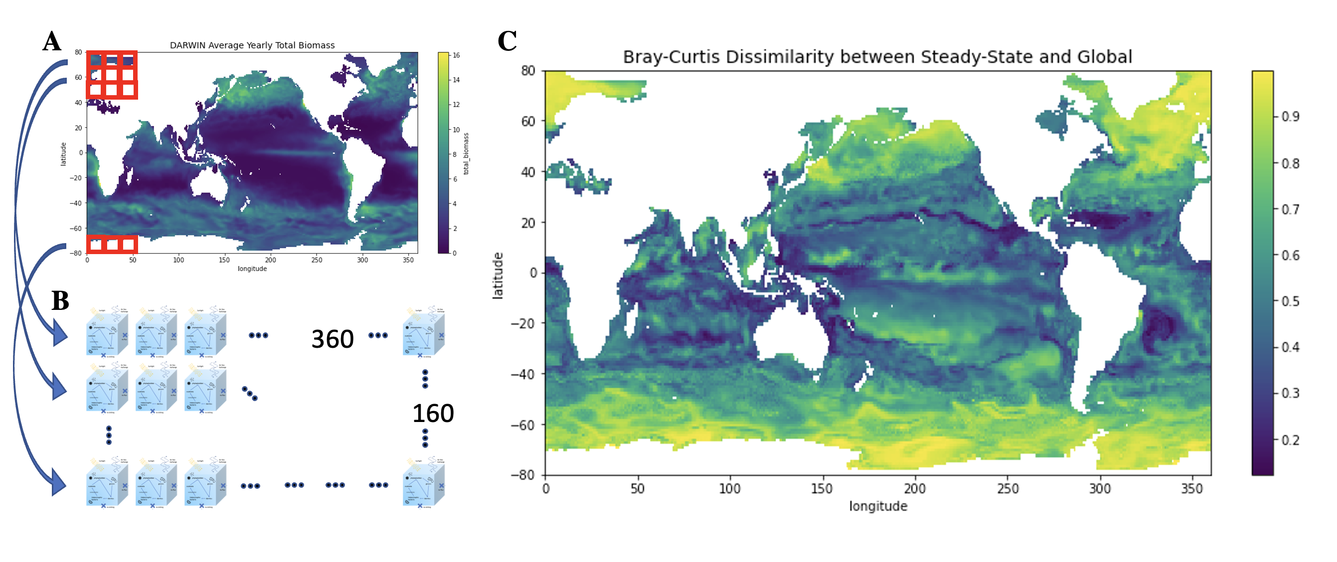
(A) The average total biomass over the course of a year in the DARWIN model. Parameters from the DARWIN model, such as nutrients, species abundance, sunlight, and temperature, are used to initialize a matrix of DAR1s, shown in (B). The DAR1 grid is 360x160 large, with each DAR1 "cell" corresponding to a lat/lon point in the DARWIN model. The grid of DAR1s is run 10 years forward, with final "steady state" values calculated from the average of the last two years. (C) shows the Bray-Curtis Dissimilarity index of the steady state community versus the initial community. The steady state is highly dissimilar to DARWIN in regions with high values (yellow), and low valued (blue) indicate areas where the community structure of the two models are comparable.

See the grid section of the beginner tutorials to learn the details of how to run DAR1 in parallel in this grid format.

Code Walkthrough

First we will open and examine the global_steadystate_build.jl file.

vim global_steadystate_build.jl

Reminder that we are in the /dar_one_docker/Dar_One/case_studies directory.

The 360 x 160 matrix was divided in 16 parts, each 90 x 40. After running, the 16 tiles were stitched together again. Prior to building, we specify this grid size, and make sure all nutients are allowed to cycle normally (i.e. the available amount in the water is not held constant)

include("../src/DarOneTools.jl")
using .DarOneTools
using NCDatasets

# set path to MITgcm 
MITgcm_path[1] = "/dar_one_docker/darwin3" # CHANGE ME (unless using docker)

# set up size of your grid
# running the 360x180 world in 16 quadrants in case something goes wrong midway
nX = 90
nY = 40

# update SIZE.h 
update_grid_size(nX, nY)

# which nutrients can change?
param_list = ones(19) # let all nutrients cycle normally
hold_nutrients_constant(param_list)

# BUILD 
build(base_configuration)

we are done with the global_steadystate_build.jl file! With vim, make sure you are not in insert mode by pressing esc then close the file by typing :q + enter.

Back in the Docker bash command line, we will run the bottle experiment build file with the command

julia global_steadystate_build.jl

A bunch of info will be printed to the console as the model is building. Just hang tight for a minute or two and wait until you see a "successful build" message.

Next we will open the global steady state run file.

vim global_steadystate_run.jl

We will go through every line of code in this file before we close it and run it from the docker command line.

The yearly averages from a global DARWIN run were used to initialize a grid of DAR1s. Here, we load up those seed files.

# load seed files - these are from global darwin runs
# yearly average!  
seed_file_3d = "/Users/birdy/Documents/eaps_research/gcm_analysis/gcm_data/darwin_yearly_avg/3d.nc"
seed_file_temp = "/Users/birdy/Documents/eaps_research/gcm_analysis/gcm_data/darwin_yearly_avg/tave.nc"
seed_file_par = "/Users/birdy/Documents/eaps_research/gcm_analysis/gcm_data/darwin_yearly_avg/par.nc"
seed_ds_3d = Dataset(seed_file_3d)
seed_ds_temp = Dataset(seed_file_temp)
seed_ds_par = Dataset(seed_file_par)
t = 1 # yearly averages, only have one timepoint

Next, we specify the ranges for breaking down the lat (y) and lon (x) into 4 sections each.

# what slice do we want?
# these are INDICES so must be INTEGERS
x_idxs = [(1,90), (91,180), (181, 270), (271,360)]
y_idxs = [(1,40), (41,80), (81, 120), (121, 160)]

for x_idx in x_idxs
    for y_idx in y_idxs
        # SEE CODE BELOW
    end
end

We initialize values and run the model inside the for loop. All of the following code goes inside that loop! First, we unpack the range values for each quadrant

        x = collect(x_idxs[x_idx][1]:x_idxs[x_idx][2])
        y = collect(y_idxs[y_idx][1]:y_idxs[y_idx][2])
        z = 1 # surface

Then set up the config files as described in the basic beginner tutorial, setting the total amount of time the model will run for to 20 years, writing to diagnostic files every 1 year, and letting the run-time files know the correct grid size.

        # set up config 
        config_id = "globe-ss-$x_idx-$y_idx"
        config_obj, rundir = create_MITgcm_config(config_name)
        setup(config_obj)

        # length of run 
        end_time = 2880*20 # 2880 is one year, in iterations
        update_end_time(config_obj, end_time)

        # output frequency 
        frequency = 2592000*12 # 2592000 is one month, in seconds 
        update_all_diagnostic_freqs(config_obj, frequency)

        # update data > PARM04 > delX and delX
        update_delX_delY_for_grid(config_obj, nX, nY)

Next we initialize all of the tracer values using the seed files, with the exception of diazotrophs which we set to zero.

        # create initial bin files for tracers that are not zero
        non_zero_tracers = cat(1:29, 35:70, dims=1)
        for tracer_id in non_zero_tracers
            tracer_name = tracer_id_to_name(tracer_id)
            init_matrix = seed_ds_3d[tracer_name][x, y, z, t]
            init_tracer_grid(config_obj, tracer_name, init_matrix)
        end

        # create initial bin files for tracers that are zero (diazotrophs)
        for tracer_id in [30,31,32,33,34]
            tracer_name = tracer_id_to_name(tracer_id)
            init_matrix = zeros(Float32, nY, nX)
            init_tracer_grid(config_obj, tracer_name, init_matrix)
        end

Lastly, we set the temperature for each grid cell according to the MITgcm Darwin yearly average, as well as the light.

        # create bin file for temperatures - all 15 degrees
        temp_matrix = seed_ds_temp["Ttave"][x, y, z, t]
        init_temperature_grid(config_obj, temp_matrix)

        # create bin files for light 
        z=3 # lower value for light - farther into the water column
        init_radtrans_grid_xy(config_obj, seed_ds_par, x, y, z, t)

Finally we can run!

        # FINALLY! Run!
        dar_one_run(config_obj)

With the run function, we are done with the global_steadystate_run.jl file! With vim, make sure you are not in insert mode by pressing esc then close the file by typing :q + enter.

Back in the Docker bash command line, we will run the bottle experiment run file with the command

julia global_steadystate_run.jl

It will take a few seconds to start up, but eventually you will see output being printed to the console.

The final "steady state" values were calculated by averaging the last 2 years.

Code to stitch the files together and calculate the bray-curtis dissimilarity score will be coming soon.

Case Study C - Nitrogen Fixers Niche

This is the experiment that inspired the ability to hold the nutients readily available in the water constant because without it nitrogen fixers might flood the system with nitrogen.

nitrogen_fixers

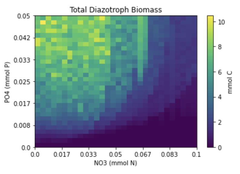
Overview

We will run a 30x30 grid of DAR1s each initialized with the same plankton community and nutrients, with the exception of nitrate and phosphate. Nitrate levels in each grid cell will increase along one axis, while phosphate levels will increase along the y-axis. Nutrient values are grabbed from the MITgcm Darwin output, but with iron at 100x and all other nutrients at 10x, and other sources of nitrogen besides NO3 (NO2, NH4, and DON) set to zero. The goal is to flood the system with nutrients, making sure it that nitogen and phosphate are the limiting factors. The simulation is run forward for 5 years with the average of the last year taken to represent the steady state result.

Code Walkthrough

From the /dar_one_docker/Dar_One/case_studies directory, we can open the nitrogenfixersbuild.jl file with vim. Because we are changing the number of grid cells we are running, we have to build the model again with these new dimensions.

vim nitrogen_fixers_build.jl

You should see the same imports at the top of the file as previously mentioned, in addition to the line MITgcm_path[1] = "/dar_one_docker/darwin3". (Reminder that you will have to point this to your local directory containing the Darwin code if you are not using the docker.)

First we update our grid size to be 30x30

# set up size of your grid 
nX = 30
nY = 30 
update_grid_size(nX, nY)

Next, we specify that we want all 19 nutrient tracers to be held constant by passing in a param list of all zeros. If we wanted to allow all nutrients to cycle normally, we would pass in a list of all ones. See the section on constant nutrients in the beginner tutorial page for more information.

# which nutrients can change?
param_list = zeros(19) # hold everything constant (0 = constant, 1=cycle)
hold_nutrients_constant(param_list)

Lastly, we call the build function with the base configuration.

# BUILD 
build(base_configuration)

Now we can close the nitrogenfixersbuild.jl file. With vim, make sure you are not in insert mode by pressing esc then close the file by typing :q + enter.

Back in the Docker bash command line, we will run the file with the command

julia nitrogen_fixers_build.jl

A bunch of info will be printed to the console as the model is building. Just hang tight for a minute or two and wait until you see a "successful build" message.

Now we will take a look at the nitrogen_fixers_run.jl file. Open it using the command

vim nitrogen_fixers_run.jl

First up in the file is the import statements for Dar1 and other packages.

Next we do the typical set-up for a DAR1 run - set the path for MITgcm to point to where the MITgcm code is, choose a unique config name for the experiment, and set up the config object.

# set path to MITgcm 
MITgcm_path[1] = "/dar_one_docker/darwin3" # CHANGE ME (unless using docker)

# create and set up config 
config_name = "n_30x30"
config_obj, rundir = create_MITgcm_config(config_name)
setup(config_obj)

After the setup step, we set the time for the simulation to run to be 5 years, in "iteration steps". (Remember: the MIT Darwin model is set up to step forward 3 hours for each iteration, so we have 8 iterations per day * 360 days = 2880 iterations per year), writing to the diagnostic files every 1 year in seconds. Running for 5 years was chosen by visually looking at longer runs of the same setup and seeing a quasi-steady state reached by that point. We write to only once a year to improve runtime performance, because we are only interested in the average values of the last year.

# length of run 
end_time = 2880 * 5 # 2880 = one year, in iterations
update_end_time(config_obj, end_time)

# output frequency 
frequency = 2592000*12 # 2592000 = one month, in seconds
update_all_diagnostic_freqs(config_obj, frequency)

We then set the entire system to have a constant temperature of 24 degrees C, and update the run-time configuration to have the appropriate grid size.

new_temp = 24
update_temperature(config_obj, new_temp)

update_delX_delY_for_grid(config_obj, nX, nY)

Then the seed files, generated by a global run of MITgcm Darwin, are loaded up to use to set initial values.

# seeded from N Pacific gyre 
seed_file = "/dar_one_docker/3d.nc"
seed_ds = Dataset(seed_file)
seed_par_file = "/dar_one_docker/par.nc"
seed_ds_par = Dataset(seed_par_file)
x = 203
y = 135
z= 1
t = 1 # using yearly averages

Next, we initialize the plankton community, excluding mixotrophic dinoflagellates. Each grid cell starts out with the same quantity of plankton. Reminder that you can see a list of all the plankton tracers, their IDs, and functional groups on the darwin backgroung page.

# start with the same plankton community in each cell 
for tracer_id in 21:70
    tracer_name = tracer_id_to_name(tracer_id)
    val = seed_ds[tracer_name][x, y, z, t]
    # no mixotrophic dinoflagellates 
    if 44 <= tracer_id <= 51
        val = 0
    end 
    init_list = repeat([val], nX)
    dim = "x"
    init_tracer_grid(config_obj, tracer_name, init_list, dim, (nX,nY))
end

The following block of code initializes the nutrients in each grid cell, with the exception of NO3 and PO4, which will be set later. Nutrient values are also grabbed from the MITgcm Darwin output, but with iron at 100x and all other nutrients at 10x, and other sources of nitrogen besides NO3 (NO2, NH4, and DON) set to zero. The goal is to flood the system with nutrients, making sure it that nitogen and phosphate are the limiting factors.

# start with the same nutrients in each cell 
for tracer_id in 1:20
    # skip no3 and po4 (2 and 5) - set later 
    if tracer_id == 2 || tracer_id == 5
        continue
    end
    tracer_name = tracer_id_to_name(tracer_id)
    val = seed_ds[tracer_name][x, y, z, t]
    # set NO2, NH4, and DON to 0 (tracers 3, 4, and 9)
    if tracer_id == 3 || tracer_id == 4 || tracer_id == 9
        val = 0.0
    end
    init_list = repeat([val], nX)
    dim = "x"
    # add TONS of iron
    if tracer_id == 6
        init_list = init_list .* 100
    else # also make everything else MORE  
        init_list = init_list .* 10
    end
    init_tracer_grid(config_obj, tracer_name, init_list, dim, (nX,nY))
end

We then set phosphate values to range from 0 - 0.05 along the y axis, keeping it constant along the x-axis, and nitrate to range from 0 - 0.1 along the x axis.

# set increasing phosphate along y axis 
tracer_name = tracer_id_to_name(5)
p_init_list = LinRange(0,0.05, nX)
dim = "y"
init_tracer_grid(config_obj, tracer_name, p_init_list, dim, (nX,nY))

# set increasing nitrate availability along x axis 
tracer_name = tracer_id_to_name(2)
n_init_list = LinRange(0,0.1, nX)
dim = "x"
init_tracer_grid(config_obj, tracer_name, n_init_list, dim, (nX,nY))

The last step before running is setting the light across the entire grid to a constant value.

# Station ALOHA(ish) light 
x = 203
y = 105
z=2 # lower value for light - farther into the water column
update_radtrans(config_obj, seed_ds_par, x, y, z, t)

Lastly we call the run function, passing it our config object that was created earlier in the file.

# FINALLY! Run! 
dar_one_run(config_obj)

Now we can close that file. With vim, make sure you are not in insert mode by pressing esc then close the file by typing :q + enter. We then run the file using the command

julia nitrogen_fixers_run.jl

It will take a few seconds for it to begin running, but you will eventually see a message indicating that the model is running, along with some warnings you can ignore. After a couple minutes, the model with finish with an obvious message saying that the run did not fail!

Output

The final output will be in the ecco_gud_DATE folder in the directory /dar_one_docker/darwin3/verification/dar_one_config/run/n_30x30/run/. In order to copy it back over to your local machine, you will need to open a terminal on your machine (NOT within the docker container) and use the docker cp command (docker cp container-id:/path/filename.txt ~/Desktop/filename.txt). You can get the container id from the docker command prompt (root@container-id:/daronedocker).

There is a 3d file created for each year we ran. We are mainly interested in the last 3d file, i.e. the 5th year (3d.0000014400.t001.nc). Here is an example of the full docker copy command.

docker cp 631c2b348d93:/dar_one_docker/darwin3/verification/dar_one_config/run/n_30x30/run/ecco_gud_20230602_0001/3d.0000014400.t001.nc ~/Desktop

Now you have a netcdf file on your local machine to explore however you prefer! In depth descriptions of all the output files can be found in Darwin Background.